How to Efficiently Retrieve Formula1 Data using FastF1 API

If, like Charles, you're seeking key heuristics for Formula 1 races, the FastF1 API (here's the documentation if you'd like to DIY) and I are here to assist you in easily accessing the latest F1 data. In this concise blog, I demonstrate how to extract data for F1 races, to report and visualize metrics such as timings, calendars, telemetry, and circuit information from all races.

Charles looking for his race heuristics!

---

Although Charles appears to be caught in an infinite loop of disappointment while seeking his race heuristics , I'll ensure that doesn't happen to you. Since I published the Formula 1 2025 Calendar Visualization on Tableau, my inbox has been inundated with inquiries from motorsports and data enthusiasts about how I obtained the data. So, without further delay, let's jump right into a simple 3-step process to create this in Tableau, with a touch of Python for data preparation and a small amount of basic Trigonometry (I promise, just a tiny bit!).

Formula1 2025 Calendar

Before I start, let’s face it, code is way more attractive than my musings—like a shiny new gadget versus a dusty old manual! Here's the complete Github Repository if you just need the code and not have any of my blabbering but if you are still interested in reading then off we go.

Take out your Jupyter notebooks or any other IDE you prefer to code in, and let's start coding:

# Importing Required Packages
import os
import fastf1  # P.S. Dont't forget to pip install if you haven't
import pandas as pd
import numpy as np
import matplotlib.pyplot as plt

Step 1: Getting the Data from FastF1 API

We fetch the data using fastf1.get_session(), specifying the 2024 Japanese Grand Prix and the qualifying ('Q') session. This helps us narrow down the data to a specific track, year, and session type. Once we have the session, we load all its available data using session.load(), ensuring we have everything we need for analysis.

Next, we select a single lap to analyze. While any lap could work, we pick the fastest lap using session.laps.pick_fastest() as it represents the best performance on the track. To visualize how the car moved during this lap, we extract its position data (lap.get_pos_data()). This gives us the exact path the car took, allowing us to map out the racing line.

Finally, we retrieve detailed circuit information with session.get_circuit_info(), which provides track layout details for Suzuka, the home of the Japanese Grand Prix. The position data is crucial because it helps us visualize the fastest lap’s trajectory, effectively mapping out the circuit layout as driven during that lap.

session = fastf1.get_session(2024, 'Japanese Grand Prix Circuit', 'Q')
session.load()

lap = session.laps.pick_fastest()
pos = lap.get_pos_data()

circuit_info = session.get_circuit_info()

---

Step 2: Trigonometry Sucks but Works!

We start by defining a function, rotate(xy, angle), which applies a rotation transformation to a set of (x, y) coordinates. The function uses a rotation matrix to adjust the points by the given angle, ensuring that the track map aligns correctly with the intended orientation.

Next, we extract the track position data from the fastest lap, specifically the X and Y coordinates, and convert them into a NumPy array. This array represents the car’s movement on the circuit.

Since the track might not be perfectly aligned for visualization, we adjust its orientation using the rotation angle provided in circuit_info.rotation. This angle is originally in degrees, so we convert it to radians (since trigonometric functions in NumPy operate in radians).

We then use the rotate() function to apply this transformation, effectively rotating the track map so it matches its correct alignment. The rotated coordinates are then converted back into a DataFrame, which we save as a CSV file (rotated_track.csv). This allows us to store the transformed track layout and use it later for visualization or analysis.

def rotate(xy, *, angle):
    rot_mat = np.array([[np.cos(angle), np.sin(angle)],
                        [-np.sin(angle), np.cos(angle)]])
    return np.matmul(xy, rot_mat)

# Get an array of shape [n, 2] where n is the number of points
# axis is x and y.
track = pos.loc[:, ('X', 'Y')].to_numpy()

# Convert the rotation angle from degrees to radian.
track_angle = circuit_info.rotation / 180 * np.pi

# Rotate and plot the track map.
rotated_track = rotate(track, angle=track_angle)

# Convert the rotated track data back into a DataFrame
rotated_track_df = pd.DataFrame(rotated_track, columns=['Rotated_X', 'Rotated_Y'])

# Save the DataFrame to a CSV file
rotated_track_df.to_csv('rotated_track.csv', index=True)

Understanding the Rotation Formula

Each new coordinate is computed as:

x′ = xcos⁡θ+ysin⁡θ

y′ = −xsin⁡θ+ycos⁡θ

This means that the x and y coordinates after rotation is influenced by both the original x and y values and the track angles, as the shape "tilts" with rotation. Track data from FastF1 might not always be aligned correctly with the expected orientation. Some tracks might be slightly tilted in their raw data, so using the provided rotate function ensures that the layout is properly oriented for visualization. This process essentially repositions the entire track while preserving its shape, making it easier to map and analyze the driving line.

If you'd like a bit more dig into the math behind how the rotation transformations work, I found this resource helpful.

---

Step 3: Extract Data and Build

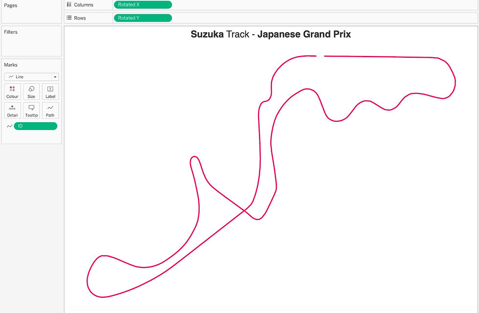
Now that we have our three essential fields- Rotated_X, Rotated_Y, and the ID field- we can easily plot the Suzuka track in Tableau. Simply place Rotated_X in the Columns shelf and Rotated_Y in the Rows shelf, then after changing the marks type to a line chart, place the ID field to Path on the marks shelf and you're all set. It’s that simple!

Plotting F1 Track in Tableau

If you're curious about how I managed to create numerous tracks in a single sheet, you can reverse engineer it using the additional code available in my GitHub repository for all_rotated_track_data, which was generated with all_track_data.ipynb. This process relies on extracting data from all tracks (including event dates from schedule) using the FastF1 API and then applying small multiples in Tableau. If you need a refresher on small multiples, check out this video here!

In my case, I created the Row and Column fields for small multiples during data preparation in Python. However, this task can also be accomplished directly in Tableau using calculations, as demonstrated in the video.

I know that this is just the beginning of what we can create with this API. I encourage you to develop more intriguing visualizations and experiment with the APIs and data. Don't hesitate to contact me on LinkedIn or X if you have any questions or want to share your use cases.

Signing Off,

Yash Sakhuja